The tutorial shows how to calculate mean in Excel for different data types by using AVERAGE or AVERAGEA formulas. You will also learn how to use the AVERAGEIF and AVERAGEIFS functions to average cells that meet certain criteria.
In plain English, calculating the average for a set of values if finding out the most common value in the set. For example, if a few athletes have run a 100m sprint, you may want to know the average result – i.e. how much time most sprinters are expected to take to complete the race.
In mathematics, average is called the arithmetic mean, or simply the mean, and it is calculated by adding a group of numbers together and then dividing by the count of those numbers.
In the above example, if the first athlete covered the distance in 10.5 seconds, the second needed 10.7 seconds, and the third took 11.2 seconds, the average time would be 10.8 seconds:
=(10.5+10.7+11.2)/3.
To calculate average in Excel, you won’t need to write such mathematical expressions, powerful Excel Average functions will do the work behind the scene. Further on in this tutorial, we will discuss the syntax of each function and illustrate it with examples of uses.
- Excel AVERAGE – calculate the mean of cells with numbers.
- Excel AVERAGEA – find an average of cells with any data (numbers, Boolean and text values).
- Excel AVERAGEIF – average cells based on a given criterion.
- Excel AVERAGEIFS – average cells that match several criteria.
- Average cells by multiple criteria with OR logic
Excel AVERAGE function
You use the AVERAGE function in Excel to return the average (arithmetic mean) of the specified cells.
AVERAGE(number1, [number2], …)
Number1, number2, … are numeric values for which you want to find the average. The first argument is required, subsequent ones are optional, and up to 255 arguments can be included in a single formula. The parameters can be supplied as numbers, cell references, or ranges.
Using the AVERAGE function in Excel – formula examples
AVERAGE is one of the most straightforward and easy-to-use Excel functions, and the following examples prove this.
Example 1. Calculating an average of numbers
To find out an average of certain numbers, you can supply them directly in your Excel average formula. For example, =AVERAGE(1,2,3,4) returns 2.5 as the result.
To calculate a column average, supply a reference to the entire column:
=AVERAGE(A:A)
To get a row average, enter the row reference:
=AVERAGE(1:A)
To compute an average of numbers in a given range, specify that range in your Average formula:
=AVERAGE(A1:C20)
To return an average of non-adjacent cells, you supply each cell individually, e.g.
=AVERAGE(A1, C1, D1)
And naturally, nothing prevents you from including values, cells references and ranges in the same formula, as your business logic requires. For example, the following average formula calculates the average of 2 ranges and 1 individual cell:
=AVERAGE(B3:B5, C7:D9, B11)
Tip. If you want to round the returned number to the nearest integer, use one of the Excel rounding functions, for example: =ROUND(AVERAGE(B3:B5, B7:B9, B11),0)

Apart from numbers, you can use the Excel AVERAGE function to calculate an average of other numeric values such as percentages and times, as demonstrated in the following examples.
Example 2. Calculating average percentage in Excel
If you have a column of percentages in your sheet, how do you get an average percent rate? By using a normal Excel formula for average 🙂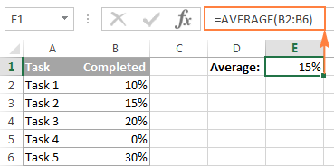
Note. Please pay attention that the Excel AVERAGE function includes zero values when calculating an average. If you’d rather exclude zeros, use AVERAGEIF instead, as demonstrated in the following example.
Example 3. Calculating average time in Excel
As you may remember, at the beginning of this tutorial, we found out the average time of three 100m sprinters with a pretty simple calculation. But what if you want to average times that include hours, minutes and seconds? Calculating different time units manually, would be a real pain… but the AVERAGE formula in Excel copes perfectly.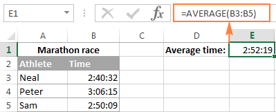
Excel AVERAGE function – things to remember!
As you’ve just seen, using the AVERAGE function in Excel is easy. However, it does have a few specificities that you need to be aware of.
- Cells with zero values (0) are included in the average.
- Cells containing text strings, Boolean values of TRUE and FALSE, and empty cells are ignored. If you want to include Boolean values and text representations of numbers in the calculation, use the AVERAGEA function.
- Boolean values that you type directly in the Excel AVERAGE formula are counted. For example, the formula =AVERAGE(TRUE, FALSE) returns 0.5, which is the average of 1 and 0.
Note. When using the AVERAGE function in Excel sheets, please do keep in mind the difference between cells containing zero values and blank cells – 0’s are counted, but empty cells are not. This might be especially confusing if the “Show a zero in cells that have a zero value” option is unchecked in a given sheet. You can find this option under Excel Options > Advanced > Display options for this worksheet.
AVERAGEA function in Excel
The AVERAGEA function is similar to Excel AVERAGE in that it calculates the average (arithmetic mean) of the values in its arguments. The difference is that AVERAGEA includes all non-empty cells in a calculation, whether they contains numbers, text, Boolean values of TRUE and FALSE, and empty strings returned by other formulas.
AVERAGEA(value1, [value2], …)
Value1, value2, … are values, arrays, cell references or ranges that you want to average. The first argument is required, others (up to 255) are optional.
Excel AVERAGEA function – things to remember!
As mentioned above, the AVERAGEA function processes different value types such as numbers, text strings and logical values of TRUE and FALSE. In AVERAGEA formulas:
- Empty cells are ignored.
- Text values, including empty strings (“”) returned by other formulas, evaluate as 0.
- The Boolean value of TRUE evaluates as 1, and FALSE evaluates as 0.
For example, the formula =AVERAGEA(2,FALSE) returns 1, which is the average of 2 and 0. The formula =AVERAGEA(2,TRUE) returns 1.5, which is the average of 2 and 1.
The following screenshot demonstrates two formulas for average in Excel and different results they return: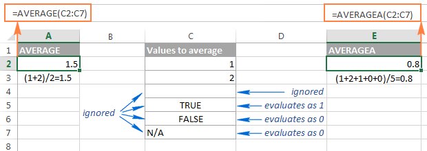
So, if you do not want to include the Boolean values and text strings in your calculations, use the Excel AVERAGE function rather than AVERAGEA.
Excel AVERAGEIF function
The AVERAGEIF function in Excel calculates the average (arithmetic mean) of all the cells that meet a specified criteria.
AVERAGEIF(range, criteria, [average_range])
The AVERAGEIFS function has the following arguments, the first 2 are required, the last one is optional:
- Range – the range of cells to be tested against the given criteria.
- Criteria – the condition used to determine which cells to average. The criteria can be supplied in the form of a number, logical expression, text value, or cell reference, e.g. 5, “>5”, “cat”, or A2.
- Average_range – the cells you actually want to average (optional). If omitted, the formula will calculate an average of the values in the range argument.
The AVERAGEIF function is available in Excel 2016, Excel 2013, Excel 2011 for Mac, Excel 2010 and 2007.
Using the AVERAGEIF function in Excel – formula examples
And now, let’s see how you can use the Excel AVERAGEIF function on real-life worksheets to find an average of cells that meet your criteria.
Example 1. Average cells that match criteria exactly
The classical use of the AVERAGEIF function in Excel is finding an average of cells that exactly match a given criterion. In this example, let’s average only the sales (B2:B8) for the Banana orders (A2:A8):
=AVERAGEIF(A2:A8, “banana”, B2:B8)
Instead of entering the condition directly in a formula, you can type it in a separate cell and refer to that cell in your formula:
=AVERAGEIF(A2:A8, E1, B2:B8)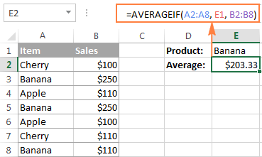
Tip. To round the returned value to a certain number of decimal places, either use one of the Excel round functions to round off the actual value stored in the cell, or the Format Cells dialog to change only the display formatting.
For example, to round the average returned by the above formula to 2 decimal places, you can wrap it in the ROUND function like this:
=ROUND(AVERAGEIF(A2:A8, “banana”, B2:B8), 2)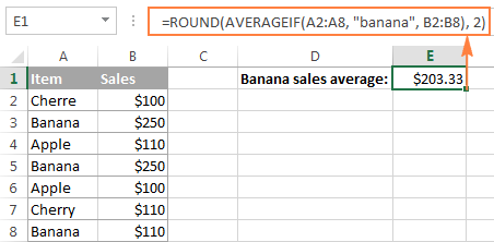
Alternatively, you can select the cell with the formula (E1 in this example), press Ctrl + 1 to open the Format Cells dialog, switch to either the Number or Currency tab and select the number of decimal places you want to display. Please remember, in this case the actual value stored in a cell won’t be changed, and the exact non-rounded value will be used in all calculations if you refer to that cell in other formulas.
Example 2. Average cells that match criteria partially (wildcard characters)
In your Excel AVERAGEIF formulas, you can use the wildcard characters in the criteria argument to average cells based on a partial match:
- Use a question mark (?) to match any single character.
- Use an asterisk (*) to match any sequence of characters.
- To find an actual question mark or asterisk, type a tilde (~) before the character in the criteria.
In the previous example, suppose you have 3 different sorts of banana and you want to find their average. The following formula will work a treat:
=AVERAGEIF(A2:A8, “*banana”, B2:B8)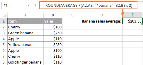
If your keyword are likely to be preceded and/or followed by some other characters, add an asterisk both in front of the word and after it, like =AVERAGEIF(A2:A8, “*banana*”, B2:B8).
To find the average of all items excluding any Banana, use the following formula:
=AVERAGEIF(A12:A18, “<>*(banana)”, B12:B18)
Example 3. Average cells based on numeric criteria and logical operators
Quite often, you may want to average cells where the quantity is greater than or less than a certain value. For example, we have a list of numbers in column A and we want to find an average of those that are greater than 10.
The correct way to enter such a criteria is to enclose the logical operator and the number in double quote. So, your formula for average in Excel would be as follows:
=AVERAGEIF(A2:A7, “>10”)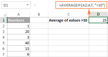
Another common task is averaging numbers that are not equal to zero. For this, you would need the “not equal to” operator in the criteria argument of your AVERAGEIF formula:
=AVERAGEIF(A2:A7, “<>0”)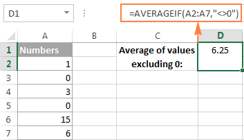
As you may have noticed, we do not use the third argument [average_range] in either of the above formulas since we want to find an average in the initial range.
Example 4. AVERAGEIF for blank or non-blank cells
When performing data analysis in Excel, you may often need to find an average of numbers that correspond either to empty or non-empty cells.
Average if blank
To include blank cells that contain absolutely nothing (no formula, no zero length string), enter “=” in the criteria argument.
For example, the following formula calculates an average of cells C2:C8 if a cell in column B in the same row is absolutely empty:
=AVERAGEIF(B2:B8, “=”, C2:C8)
To average values corresponding to visually blank cells including those that contain empty strings returned by other functions (for example, cells with a formula like =””), use “” in criteria. For example:
=AVERAGEIF(B2:B8, “”, C2:C8)
Average if not blank
To find an average of values corresponding to non-empty cells, type “<>” in criteria.
For instance, the following AVERAGEIF formula calculates an average of cells C2:C8 if a cell in column B in the same row is not blank:
=AVERAGEIF(B2:B8, “<>”, C2:C8)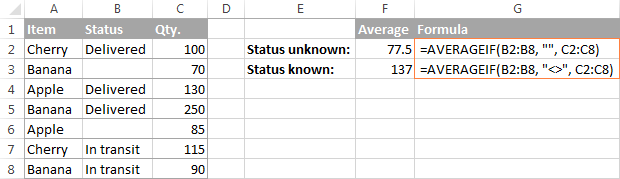
Example 5. Using cell references and other functions in AVERAGEIF’s criteria
Instead of typing the criteria in a formula, you can refer to a certain cell where your users can input different values without altering your AVERAGEIF formula.
In case a cell reference is an exact match criteria, simply type it in the criteria argument like we did in Example 1:
=AVERAGEIF(A2:A8, E1, B2:B8)
If you use a logical expression with a cell reference or another function in criteria, then you have to enclose the logical operator in “double quotes” and add ampersand (&) to concatenate a cell reference or function.
For example, to calculate average sales (C2:C8) that are greater than the value in E4, use the following formula:
=AVERAGEIF(C2:C8, “>”&E4)
With dates in B2:B8, the below formula returns the average of sales (C2:C8) that we made up to the current date:
=AVERAGEIF(B2:B8, “<=”&TODAY(), C2:C8)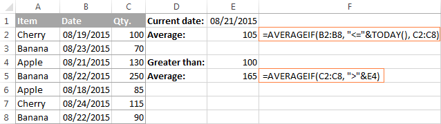
Excel AVERAGEIFS function
The AVERAGEIFS function in Excel is a plural counterpart of AVERAGEIF. It allows for multiple conditions and returns the average (arithmetic mean) of cells that meet all of the specified criteria.
AVERAGEIFS(average_range, criteria_range1, criteria1, [criteria_range2, criteria2], …)
The AVERAGEIFS function has the following arguments:
- Average_range – the range of cells that you want to average.
- Criteria_range1, criteria_range2, … – 1 to 127 ranges to be tested against the specified criteria. Criteria_range1 is required, subsequent ones are optional.
- Criteria1, criteria2, … – 1 to 127 criteria that determine which cells to average. The criteria can be supplied in the form of a number, logical expression, text value, or cell reference. Criteria1 is required, additional criteria are optional.
The AVERAGEIFS function is available in Excel 2016, Excel 2013, Excel 2011 for Mac, Excel 2010 and 2007.
Excel AVERAGEIFS formula examples
As already mentioned, the Excel AVERAGEIFS function finds average of cells that meet all of the criteria that you specify (AND logic). In essence, you use it similarly to AVERAGEIF, except that you can supply more than one criteria_range and criteria in a formula.
Example 1. Average cells by multiple criteria (text and number)
Supposing that you have a list of items in column A and sales amounts in column B, let’s find out an average of Banana sales that are greater than $100.
In this AVERAGEIFS formula:
- Average_range is B2:B8 (cells that you want to average if both conditions are met);
- Criteria_range1 is A2:A8 (Items column) and criteria1 is “banana”;
- Criteria_range2 is B2:B8 (Sales column) and criteria2 is “>100”.
By assembling the above components together, we get the following formula:
=AVERAGEIFS(B2:B8, A2:A8, “banana”, B2:B8, “>100”)
And if you replace the actual values with cell references in your formula, you will get something similar to this: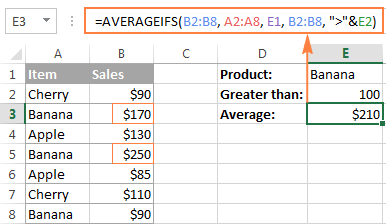
As you see, only two cells (B3 and B5) meet both conditions, and therefore only these cells are averaged.
Example 2. Average cells based on date criteria
In this example, let’s find an average of items delivered prior to 21-Aug-2015 whose status is defined (a cell in the corresponding column is not empty). With quantity listed in column D (average_range), dates in column B (criteria_range1) and status in column C (criteria_range2), the formula is as follows:
=AVERAGEIFS(D2:D8, B2:B8, “<8/21/2015”, C2:C8, “<>”)
In criteria1, you enter a date preceded with a comparison operator. In criteria 2, you type “<>” that tells the formula to include only non-empty cells within citeria_range2 (column C in this example).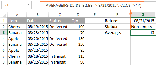
Tip. When you use a number or date in conjunction with a logical operator in AVERAGEIFS’ criteria, you enclose this combination in double quotes like “<8/21/2015”.
AVERAGEIF and AVERAGEIFS functions – things to remember!
Excel AVERAGEIF and AVERAGEIFS functions have much in common, in particular:
- In the average_range argument, empty cells, Boolean values of TRUE/FALSE and text values are ignored.
- In the criteria / criteria_range argument, empty cells are treated as zero values (0).
- If average_range contains only blank cells or text values, both functions return the #DIV0! error.
- If not a single cell meets the criteria (all of the criteria in case of AVERAGEIFS), the #DIV0! error is also returned.
AVERAGEIF specificities
- Average_range does not necessarily have to be of the same size as range. However, the actual cells to be averaged are determined by the size of the range argument. In other words, the upper left cell in average_range is treated as the beginning cell, and includes as many columns and rows as contained in the range argument.
AVERAGEIFS specificities
- Unlike the AVERAGEIF function, AVERAGEIFS requires each criteria_range to be of the same size as average_range.
How to average cells by multiple criteria with OR logic
Since the Excel AVERAGEIFS function works with the AND logic and the AVERAGEIF function allows for 1 criterion only, we will have to make up our own formula to average with the OR logic. In other words, we will make a formula to calculate average in Excel if any of the specified conditions is met.
Example 1. Average with OR logic based on multiple text criteria
Supposing you want to get a sales average (C2:C8) both for banana and apple (A2:A8). To calculate this, you would need an array formula comprising a few Excel functions:
=AVERAGE(IF(ISNUMBER(MATCH(A2:A8, {“banana”, “apple”},0)), B2:B8))
Please remember that array formulas need to be entered via Ctrl + Shift + Enter, not just ENTER.

Of all Excel average formulas discussed so far, this is the trickiest one (though, there are two more examples left 😉 The following pattern will make it easier to adjust the formula for your own worksheets:
=AVERAGE(IF(ISNUMBER(MATCH(range, {“criteria1“, “criteria2“,…}, 0)), average_range))
Example 2. Average with OR logic based on numeric criteria with comparison operators
If you want to average cells based on several numeric criteria and greater than / less than conditions combined with OR logic, the formula discussed in the previous example won’t work because you cannot fit those logical expressions into an array. The solution is using the SUM function in an array formula.
Supposing you have Qty. in column B and Sales in column C, and would like to average Sales that have a value greater than 50 either in column B or C. At that, you want to avoid duplicates, i.e. don’t count a row twice because it has value greater than 50 both in column B and D.
Here’s the formula that works a treat:
=SUM(IF(–((C2:C8>50)+(D2:D8>50))>0,D2:D8,0)) / SUM(–(((C2:C8>50)+(D2:D8>50))>0))
Remember, it’s an array formula, and therefore you should press Ctrl + Shift + Enter to enter it correctly.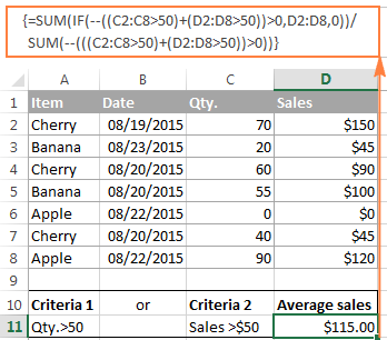
As you can see, the formula consists of 2 parts. In the first part, you use the IF function with the OR statement in the logical_test argument (C2:C8>50)+(D2:D8>50). As you probably know, in array formulas, plus (+) acts like an OR operator (for more details, please see AND and OR operators in Excel array formulas). So, the first part of the formula adds up the values in column C if either condition is met. The second part returns the count of such cells, and then you divide the sum by the count to find the average.
And naturally, you can specify a different condition for each range. For example, to average sales if column C is greater than 50 or column D is greater than 100, use the following expressions: (C2:C8>50)+(D2:D8>100). The entire formula would look as follows:
=SUM(IF(–((C2:C8>50)+(D2:D8>100))>0,D2:D8,0)) / SUM(–(((C2:C8>50)+(D2:D8>100))>0))
Example 3. Average with OR logic based on blank / non-blank cells
The average formula with multiple OR criteria corresponding to blank and non-blank cells is very similar to the one we have just discussed.
Formula for non-blank cells
The following array formula finds the Qty. average (column B) if either a date (col. B) or status (col. C) is listed, i.e. if column B or C is not empty.
=SUM(IF(–((B2:B8<>””) + (C2:C8<>””))>0,D2:D8,0)) / SUM(–(((B2:B8<>””) + (C2:C8<>””))>0))
To make the formula more compact, you can concatenate the ranges using an ampersand (&):
=SUM(IF((B2:B8&C2:C8)<>””,D2:D8,0)) / SUM( –((B2:B8&C2:C8)<>””))

Formula for blank cells
To average values in column D corresponding to empty cells either in B or C, replace the non-blank operator (<>””) with blank operator (=””). Concatenating the ranges with an ampersand won’t work in this case. This is also an array formula, so remember to press Ctrl + Shift + Enter, not just Enter.
=SUM(IF(–((B2:B8=””) + (C2:C8=””))>0,D2:D8,0)) / SUM(–(((B2:B8=””) + (C2:C8=””))>0))
This is how you calculate average in Excel. For better understanding of the formulas, feel free to download the Excel Average worksheet. In the next article, we will discuss a couple of formulas find weighted average in Excel and you might be surprised to know that it’s much easier than it sounds. I thank you for reading and hope to see you on our blog next week!